What machine learning can predict: a number, a category, a group, a preference, the next word
CS 2010 — Computing Fundamentals
2026-11-18
One question, six shapes
Machine learning is not one technique. It is a family of ways to fill in a blank — and the shape of the answer decides the method.
you want to predict
the shape of the answer
the method
how much?
a number
regression
which one?
a category
classification
what groups?
a group
clustering
what structure?
a simpler picture
PCA
what will you like?
a preference
recommendation
what comes next?
the next thing
generation
Every one of them gets the same four slides: what the problem is, how the approach works, whether it helps, and one example followed all the way through.
Part 0 — The Map
A model is fit to examples
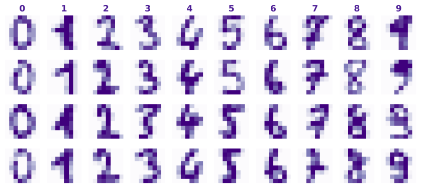
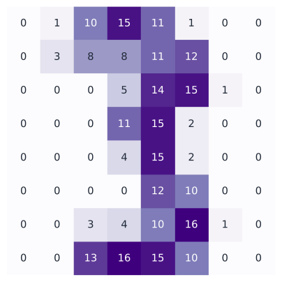
An 8 × 8 image is 64 numbers — the features.
The digit 0–9 is the label. One row is one example.
We hide the answers for 30% of the data. The only honest score is on the 540 digits the model never saw.
A classifier is a function from 64 numbers to one of ten labels.
Every model makes the same three calls
from sklearn.neighbors import KNeighborsClassifiermodel = KNeighborsClassifier(3)model.fit(X_train, y_train) # learn from the answersmodel.predict(X_test) # guess the held-back examplesmodel.score(X_test, y_test) # 0.985
fit — learn from examples.
predict — answer for new ones.
score — check the answers.
A line, a tree, a clustering, a recommender: the same three calls.
Monday’s six verbs become these three.
Always beat the dumb baseline
The most common digit is 3 — 183 of the 1,797 examples.
A “classifier” that always answers 3 is right 10.2% of the time.
For a regression, the dumb baseline is the mean.
If 1% of your email is spam, “never spam” is 99% accurate and completely useless.
Accuracy alone is a liar. Every real model has to beat the dumb baseline first.
Part I — A Number
How much will this table tip?
The problem
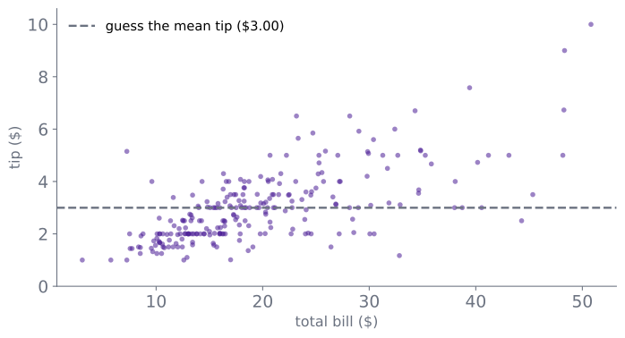
A restaurant wants to know how much this table will tip, before the bill is paid. The answer is a number, and the guess has to be close enough to plan with.
The dumb answer is the average tip — the dashed line. It is right on average and wrong for every individual table.
Why a line?
Why this method?
The answer we want is a number, and the one thing we know is another number. The simplest rule that turns one into the other is a line: two numbers describe it completely, and it can be checked against every table we have.
Anything fancier — a curve, a tree, a network — has to beat this line before it is worth the trouble. So the line is not a toy: it is the standard the rest have to clear.
A line is a rule
The approach
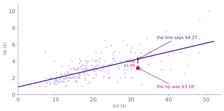
Fit a straight line through the cloud:
tip ≈ 0.92 + 0.105 × bill
That formula is the model. Give it a bill, it gives back a tip:
bill
the line says
$10
$1.97
$30
$4.07
$50
$6.17
Two numbers describe the whole line:
slope 0.105 — each extra $10 of bill adds about $1.05 to the guess.
intercept 0.92 — the guess for a $0 bill, which is nonsense, and a sign the line is only meant for the range we saw.
Regression: predicting a number from other numbers, by fitting a rule that is as close as possible to the examples.
How the line is chosen
The approach
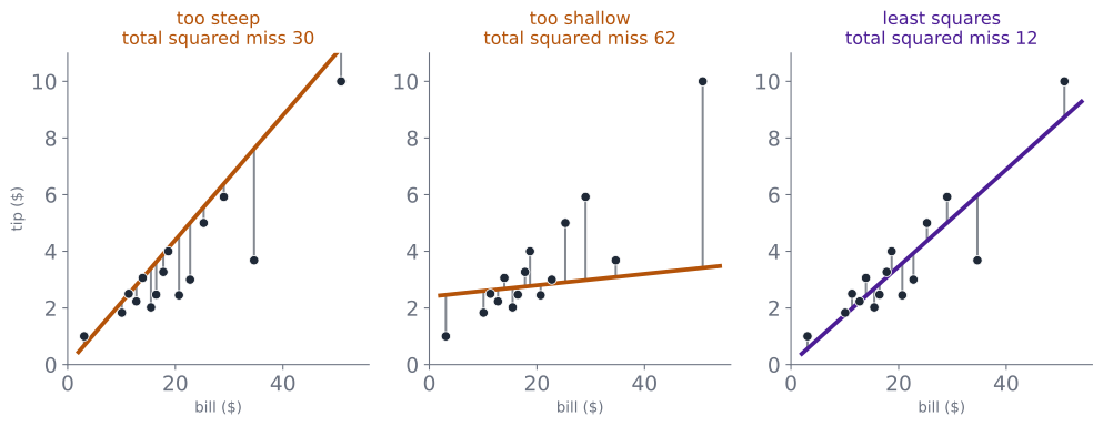
For every dot, the miss is the vertical gap to the line. Square each miss, so a miss above and a miss below do not cancel. Add them up.
The line with the smallest total wins. That is all “least squares” means.
Does it help?
Does it help?
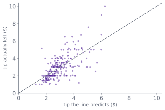
Against the mean, the line earns its keep:
typical miss
guess the mean
$1.38
use the bill
$1.02
R² = 0.46: the line explains 46% of the variation in tips. The other 54% is everything the bill does not know — the service, the weather, the party.
A model that cannot beat the mean has found nothing.
One table, end to end
An example
A table with a $31.85 bill. The line says the tip will be $4.27. The tip was $3.18 — a miss of $1.09, about the typical miss.
That is the whole method: one row in, one number out, and a miss you can measure.
The same line with a calendar
An example
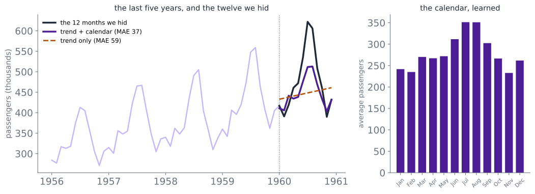
Now the number is passengers next month, and one feature is the month. A trend alone misses the summer peak; the month fixes it.
Trend only: off by 59. Same month last year: 48. Trend + calendar: 37.
Part II — A Category
Which digit is this?
The problem
A classifier predicts a category: spam or not, sick or well, which digit.
The input is still a row of numbers. A digit is 64 pixels, each 0–16.
The model never hears the word “stroke”. It gets 64 numbers and has to find the pattern — and the same digit looks different every time somebody writes it.
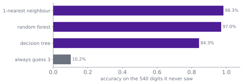
The dumb answer here is “always say 3”, which is right 10.2% of the time.
There is no formula for “looks like a 3”
Why this method?
We cannot write a rule that turns 64 pixel values into “3”. Nobody can say which pixels matter, and the same digit is written differently every time.
What we do have is 1,257 examples with the answers attached. So every method in this part works the same way:
Compare the new digit with stored examples, and let the comparison decide.
Three different comparisons, three methods: the nearest example, a series of pixel questions, and a crowd of question-askers.
The dumbest classifier that works
The method
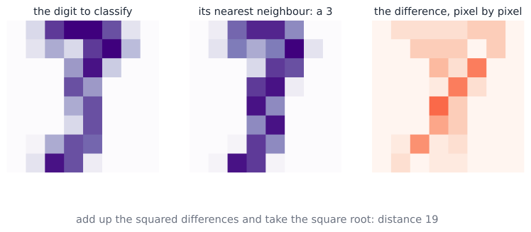
Keep every training digit. To classify a new one, measure how far it is from each digit you already have, and copy the label of the closest.
Distance is the ordinary straight-line distance across the 64 pixels: add up the squared difference in each pixel, then take the square root.
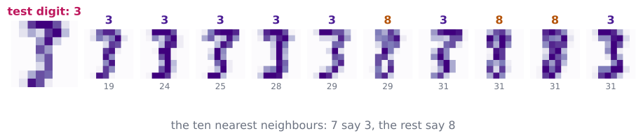
The closest of the 1,257 training digits differs by a distance of 19 — under a third of a shade per pixel. Two handwriting samples that close should be the same digit.
Let the nearest ten vote
The method
One neighbour is a fragile answer: a single odd digit can decide everything. So take the k closest and let them vote — here, the ten closest.
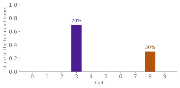
Seven say 3. Three say 8. The answer is “3, with 30% doubt”.
A tree asks one pixel at a time
The method
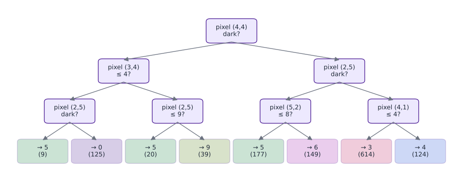
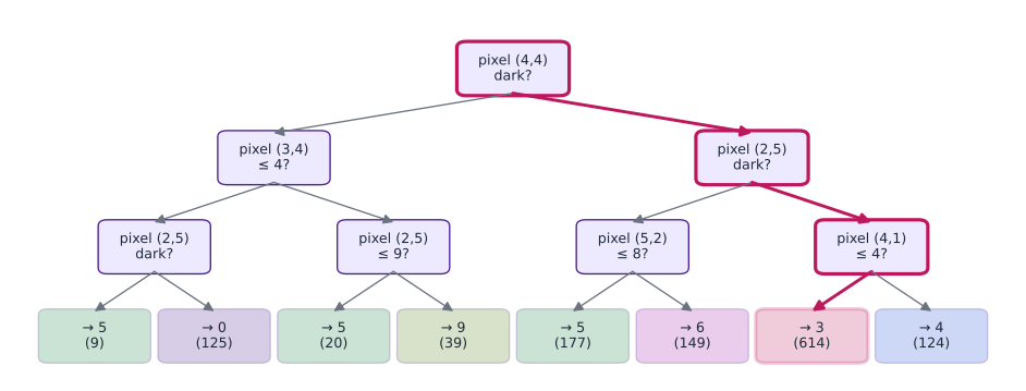
Each box is a yes/no question about one pixel. Follow the answers down the branches; the leaf you land in is the answer, with the number of training digits that landed there.
It is built greedily: try every pixel and every threshold, keep the question that separates the two piles best, then repeat on each side with the digits that went that way.
The same digit, a different answer
An example
Three questions deep, the tree lands in a pile of 614 training digits: 115 threes and 115 eights. It is a tie, broken by an arbitrary rule. It says 3 — and it is right by luck.
Let the tree keep splitting until every leaf holds a handful of digits, and the same 3 lands in a leaf of two training digits, both 8s. It says 8, with no doubt at all.
Where it stops helping
Where it stops helping
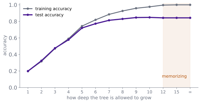
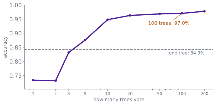
A tree three questions deep gets 47.6% — too simple. Unlimited depth gets 100% on the data it trained on and 84.3% on the data it never saw.
That gap is overfitting: the model learned the examples, not the pattern. The previous slide is the extreme case — a leaf with two training digits in it.
A hundred trees, each a little wrong
The method
Grow a hundred trees. Each one sees a random sample of the rows — some digits twice, some not at all — and each split may only look at a random handful of pixels.
So each tree asks different questions. Three of them, on the same 3:
tree
its first question
its answer
1
is pixel (4,4) dark?
9
2
is pixel (3,6) dark?
3
3
is pixel (2,5) dark?
3
Two to one for 3. Let all hundred vote.
Why the crowd wins
Does it help?
One deep tree gets 84.3%. A hundred deep trees, each on a different sample, average to 97.0% — a random forest.
The individual trees are still wrong as often as before. Their mistakes are just in different places, so the vote cancels them.
Does it help?
Does it help?
model
what it is, in one line
nearest neighbour
copy the closest example
decision tree
twenty yes/no questions about pixels
random forest
a hundred trees voting
The dumb answer is 10.2%; every real model is above 84%; the gap between the simplest and the fanciest is about 13 points.
One digit, end to end
An example
The test digit is a 3. Ten neighbours vote, and this is the tally.
The answer is “3, with 30% doubt”.
The doubt is not decoration. It is a distribution over the ten digits — and the last part of this lecture is what you can do with one.
Part III — A Group
What groups are in here?
The problem
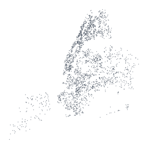
Four thousand 311 calls, each with a (latitude, longitude). Nothing else.
Nobody tells us which calls are Bronx and which are Brooklyn. There is no label to predict, and no answer to check against.
The question is: does this cloud have parts?
Why distance?
Why this method?
There are no labels here, so nothing can be right or wrong, and nothing can be scored. The only thing we can measure is how far apart two points are.
So “group” has to mean “points that are close to each other”, and the method has to be a way of finding clumps of closeness. Distance is not a choice we made; it is the only evidence in the file.
A group is points that are close together
The approach
Two points are close if the straight-line distance between them is small.
A good set of groups is tight inside and far apart between: points in the same group should be near each other, and the groups should not overlap.
We choose the number of groups k. There is no correct k — only a defensible one.
Clustering: finding groups in data when nobody has told you what the groups are.
The loop
The approach
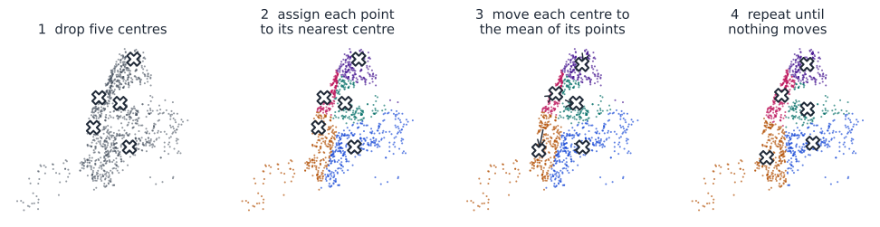
Drop k centres at random. Assign every point to its nearest centre. Move each centre to the mean of its points. Repeat until nothing moves.
Does it help?
Does it help?
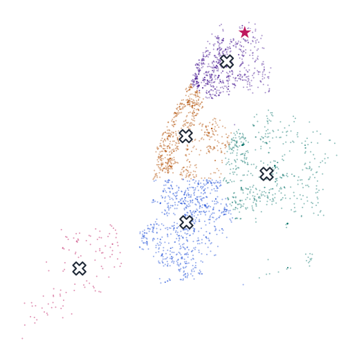
Five groups, from nothing but coordinates.
The five patches are the city’s density, and they land close to the boroughs — nobody told it about geography.
They are not the boroughs: a cluster is a patch of dense calls, and a borough is a government. The model found structure, not meaning.
How many groups?
Does it help?
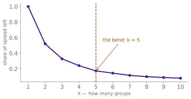
The curve shows how much spread is left after k groups. It always falls; the question is where it stops falling fast.
The bend is around 4–6. We chose 5 because the city has five boroughs — a judgement, not a law.
One address, end to end
An example
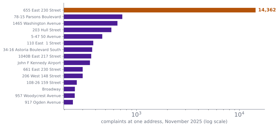
One address filed 14,362 complaints in November. The next filed 728. That is a 20× gap.
Same idea, one number per point: model what normal looks like, then flag what is far from it.
Part IV — A Picture
64 numbers is too many
The problem
A digit is a point in 64-dimensional space. You cannot draw that, and neither can I.
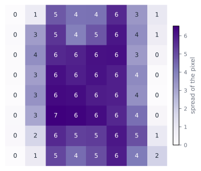
Most of the 64 numbers are redundant. The spread of each pixel across all 1,797 digits is on the right: the border barely moves, so it cannot help tell one digit from another.
We want fewer numbers that keep most of the structure.
Why the directions of spread?
Why this method?
We have to keep fewer numbers, so we have to decide which ones to throw away. A column that is the same for every digit — the border — tells us nothing. A column that moves in step with another one is redundant.
So the numbers worth keeping are the directions in which the data actually varies. That is the whole idea of a principal component.
A new axis is a combination
The approach
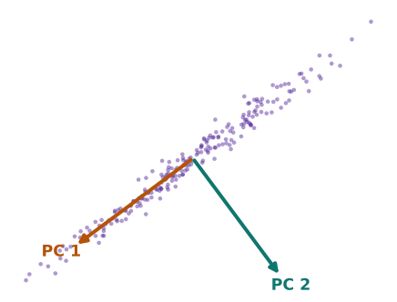
Centre the data, then find the direction in which it spreads the most. That is the first component — the longest shadow of the cloud.
The second component is the longest direction at right angles to the first.
Each component comes with a share of the variance: how much of the spread it carries.
Principal component analysis: replacing many correlated columns with a few new ones, built as weighted combinations of the originals.
The shadow
The approach
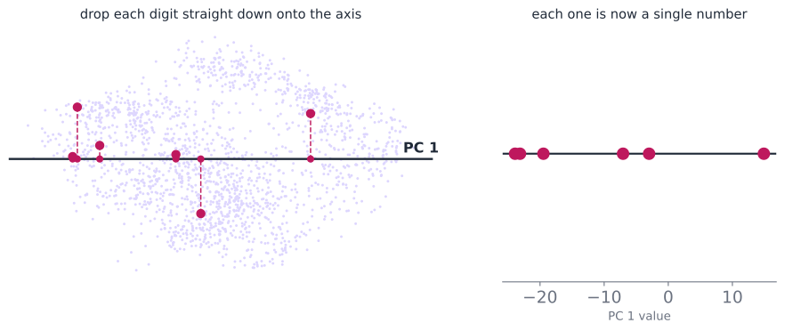
Drop every digit straight down onto the first component: each one becomes a single number.
That is all a component does — it throws information away on purpose, and keeps the part that varies most.
Does it help?
Does it help?
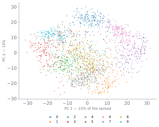
Two numbers per digit instead of 64.
The digits form islands: similar digits land near each other. But the islands overlap — a 2-D shadow cannot separate ten handwriting styles.
Two components carry 28.5% of the spread, so this is a lossy summary, not the data.
Ten numbers instead of 64
An example
Keep k components, then rebuild the image from them.
One component: 15% of the spread. Ten: 74%, and the digit is readable. Forty: 99%.
Part V — A Preference
A table with holes in it
The problem
A recommendation predicts a preference: a rating, a click, a song.
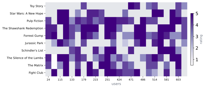
The data is a matrix, not a table: users down one side, films down the other, and most cells are empty. 149 of 240 here.
The question is the missing cell: what would this user give this film?
Why other people’s ratings?
Why this method?
We want to fill a cell nobody filled. There is no rule that turns a user and a film into a rating.
The only evidence in the file is what other people said about the same film — and the useful ones are the people whose taste already matches. So the method has to be: find those people, and average what they said.
People like you
The approach
Find the users whose ratings look most like yours, and let them vote on the film you have not seen.
Similarity is computed only over films both users rated — otherwise a user who rated everything would look similar to everyone.
Each user’s ratings are centred first: a harsh grader and a generous one can still agree.
For user 215 and Fight Club:
neighbour
similarity
their rating
581
0.94
4.5
211
0.78
5.0
471
0.76
4.0
419
0.70
5.0
111
0.62
5.0
The weighted average
The approach
Each neighbour’s rating is multiplied by their similarity; the total is then divided by the total similarity.
neighbour
similarity × rating
581
0.94 × 4.5 = 4.23
211
0.78 × 5.0 = 3.90
471
0.76 × 4.0 = 3.04
419
0.70 × 5.0 = 3.50
111
0.62 × 5.0 = 3.10
total
17.77 ÷ 3.80 = 4.68
A neighbour who agrees with you more gets more of the vote — that is the “weighted” part.
The nearest neighbour alone would have said 4.5. The crowd says 4.68.
That is the whole of user-user collaborative filtering.
Does it help?
Does it help?
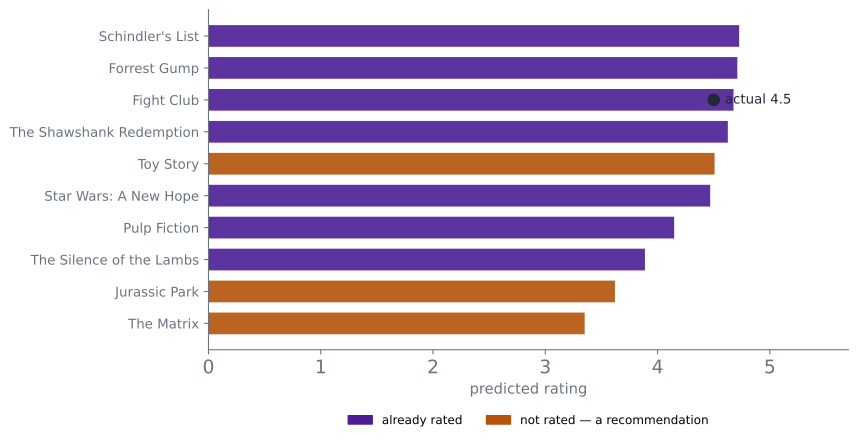
Fight Club was predicted at 4.68; the actual rating was 4.5. We hid a rating we knew and got it back to within a fifth of a point.
The violet bars are films already rated — the check. The orange ones are the recommendations: films user 215 has not seen.
A new user has no ratings
An example
A new user has rated nothing. A new film has been rated by nobody.
Every method on the previous slides needs other people’s opinions, and for a brand-new user or film there are none. That is the cold start, and no amount of matrix arithmetic fixes it.
The fixes are not arithmetic: ask the new user a few questions, or use content features — genre, cast, text.
Part VI — The Next Thing
What comes next?
The problem
Some answers are sequences: the next character, the next word, the next frame of a film.
A single label is not enough here. After “lord,” there are many characters that could come next, and several of them are reasonable.
What we want is not one answer but the whole set of answers with their chances — a distribution.
Distribution: the possible answers, with the share of the time each one happens. A histogram is one; a list of percentages is one.
Why counting?
Why this method?
We want the next character. There is no rule that says what follows “lord,”.
The only evidence is what followed it last time. So we count, over every context in a million characters, and let the counts be the model. When we meet a context we have never seen, we fall back on how often each character appears at all.
Count what follows
The approach
Train on 1 MB of Shakespeare. For every six-character context, count which character came next.
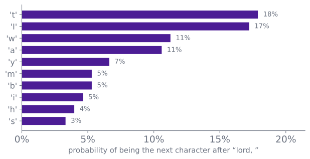
This is one row of that table: after “lord,” the next character was “t” 18% of the time, “I” 17%, “w” 11%, and so on.
Fit means count. Predict means look up the row.
Two ways to read the row
The approach
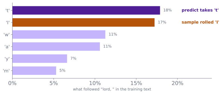
Predict takes the tallest bar: the answer is “t”.
Sample rolls a weighted die: take a bar at random, with taller bars more likely to win. This time it came back with “I”.
Same row, same numbers. One is a decision, the other is a draw.
Does it help?
Does it help?
Six characters of context, 65 possible next characters.
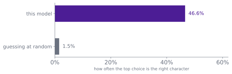
It gets the next character right 46.6% of the time. Guessing at random would be about 1.5%.
That is not a good language model by modern standards. It is a perfectly good classifier — and everything in the next two slides is the same table, read differently.
Sample it and it writes
An example
ROMEO:
A gentle ears.

Provost:
I am disgracious lord, I will not out a word.

PRINCE EDWARD IV:
What she shall see us richly in the come to the people in
a command. I was bad into a poor dukedom, through the southern lords, thou art a villain in love,
Predict a distribution → sample one character → append → repeat.
It is not retrieving Shakespeare. It is guessing, then guessing again, 245 times.
One distribution, two directions
The claim
this model
a modern language model
context
6 characters
~100,000 tokens
choices
65 characters
~100,000 tokens
parameters
a few million counts
hundreds of billions
training text
1 MB
trillions of tokens
The operation is identical: P(next thing | context). Only the scale changed.
To tell things apart well, a model ends up learning how they are made.
Part VII — The Discipline
Accuracy is not enough
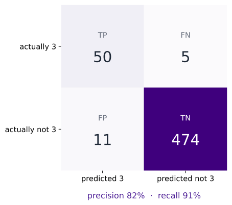
Ask a narrower question: is this digit a 3?
There are 55 threes in 540 test digits. “Never a 3” is 89.8% accurate — and finds none of them.
Precision: of the digits we call 3, how many are 3? 82%
Recall: of the real 3s, how many did we find? 91%
Features are the real work
The model sees numbers. Your table is not numbers yet.
raw
encoded
why
day = "Sat"
day_Sat = 1, others 0
a model cannot multiply a word
bill = 42.7
(bill − mean) / sd
keep one big column from dominating
smoker = "Yes"
smoker = 1
two categories become one column
"no heat in apartment"
counts of 4,000 words
text becomes a row of numbers
missing age
median, or a “missing” flag
a blank is information too
Most of the work in a real project is this column, not the model.
The model learns our biases
A model learns the world in the data, including its unfairness.
Feedback loops: more policing in a neighbourhood records more crime, which sends more police there.
Proxy features: zip code stands in for race; a resume model learns the hiring history, not the job.
Privacy: a model that predicts a person is also a model that knows something about them.
The model is not neutral because it is arithmetic.
Part VIII — Wrap
The map
you want
the method
reach for it when
a number
regression
the answer is a quantity
a category
classification
the answer is one of a few labels
a group
clustering
there are no labels
a simpler picture
PCA
the table is wide and correlated
a preference
recommendation
the data is a users × items matrix
the next thing
generation
the answer is a sequence
Start with the shape of the answer. The method follows.
Five things to remember
The shape of the answer decides the method.
Score on data the model never saw; beat the dumb baseline.
Simple methods are close to fancy ones. The boundary is the thing.
Overfitting is memorizing; the train/test gap is the symptom.
Classification and generation are two directions of one probability model.
Where this goes
Monday: k-means found groups with no labels at all.
Today: the shape of the answer — number, category, group, picture, preference, next thing.
Next: the labels dissolve again, and the model learns the data itself.
The same three calls — fit, predict, score — run a line, a tree, a recommender, and a trillion-parameter model.
The lab: build the six, break the tree, sample the text.