Caches and the Memory Hierarchy

The stock story, and what four real cores did with it

CS 4250 — Computer Architecture

2026-10-19

Roadmap

Six parts. Parts I–IV are the standard story — the one in any textbook. Parts V–VI are about the four cores on the desk in front of you.

The stock story

1. Why a hierarchy exists — the technology, and the economics
2. Locality — the empirical fact that makes it work
3. AMAT — the one equation
4. The mechanisms — direct-mapped, block size, associativity, replacement, write policy

Our silicon

5. Four cores, four answers — C906 ×2, Cortex-A53, Ryzen 7 9850X3D
6. Synthesis

Frame the deck: two halves, and the second half is why the first half is worth learning. Everything in Parts I–IV will be tested; everything in Part V is what makes it stick, because it is about the chip in their hand.

Do not let the deck become a tour of MIT’s slides. Every mechanism gets taught from scratch, then immediately grounded in our hardware.

Part 0 — Framing

The Gap

A core at 1 GHz retires an instruction every 1 ns. That is the clock we build the pipeline around. Now look at what memory costs:

Level	Latency	In 1 GHz core cycles
Register file	~0	0
L1 SRAM	1–4 ns	1–4
L2 (A53 only)	~10 ns	~10
DDR3, random access	60–100 ns	60–100
SPI NAND, page read	50–100 µs	50,000–100,000

A program that missed on every access would run a hundred times slower than the core is capable of. No amount of pipelining, branch prediction, or superscalar width fixes that — the core would simply sit idle.

The 1 ns figure is the whole motivation. Say it out loud: “the CPU can start a new instruction every nanosecond, and DRAM takes a hundred.”

Note the last row: SPI NAND is five orders of magnitude off the core. That is why “just put the program in flash and run it” does not work, and why everything gets copied into DRAM at boot — which they saw in the boot deck.

Caveat to state honestly: the DDR3 number is an estimate from CAS latency plus tRCD plus controller overhead, not a measurement. We will come back to it in Part III.

What a Level Must Buy

Every storage technology is characterised by four numbers. The MIT table, with ours alongside:

	Capacity	Latency	Cost per bit	On our board
Registers	1000s of bits	20 ps	$$$$	31 × 64 b + PC
SRAM	10 KB – 10 MB	1–10 ns	$$$	96 KB of L1
DRAM	~10 GB	80 ns	$	512 MB DDR3
Flash	~100 GB	100 µs	¢	16–64 GB NAND
Disk	~1 TB	10 ms	¢	eMMC, up to 2 TB

Read the table down the columns: every step down is roughly 10× more capacity for 10× more latency and 10× less cost per bit. That is not a coincidence of engineering — it is the physics of how you store a bit.

This is MIT’s slide 2/14 table, relabelled with our hardware. The point to land: the trade is remarkably consistent across five orders of magnitude. Which means it is a law, not a product decision.

The “cost per bit” column is the one students skip. Make them read it: DRAM is ~1000× cheaper per bit than SRAM. That is the reason a 512 MB SRAM does not exist, and no amount of cleverness will make one.

The Promise

The hierarchy is not a memory. It is an illusion generator: a small, fast, expensive memory that behaves like a large, fast, cheap one.

Three claims, and the rest of the lecture is support for them:

1. A large fast memory cannot be built. (Part I)
2. Programs have locality, so a small fast memory suffices. (Part II)
3. We can quantify how well it works, and tune it. (Parts III–IV)

Claim 2 is the one that could have been false. It is an empirical fact about real programs, not a theorem — and it is the fact the entire memory hierarchy rests on.

Flag claim 2 hard. If programs accessed memory uniformly at random, caches would buy exactly nothing, and every technique in this lecture would be pointless. Locality is the load-bearing assumption.

It is also an assumption programmers can break, and do — which is why the later material on conflict misses and working sets matters.

What We Will Not Do Today

• Virtual memory. Translation, page tables, page faults — that is a later deck. We will only touch the MMU where it forces a cache design decision.
• Coherency. Multiple cores, multiple caches, who wins. Named, not solved.
• The lab. How you measure any of this on the board is a separate conversation.

What we will do: build the whole standard model from the transistor up, and then check it against four real cores — two of which are on the same die and disagree with each other.

Scope-setting. Students will ask about virtual memory immediately because the C906 has an MMU and a TLB; defer it explicitly.

The “two cores on the same die disagree” line is the hook for Part V. Do not explain it yet.

Part I — Why a Hierarchy Exists

Four Ways to Store a Bit

Everything below follows from how many devices it takes to hold one bit.

	Devices per bit	Access time	Volatile	Writes
SRAM	6 transistors	1–10 ns	yes	unlimited
DRAM	1 transistor + 1 capacitor	~80 ns	yes	unlimited
Flash	1 floating gate	10–100 µs	no	~10³–10⁵, then worn out
Disk	a magnetic domain	10 ms	no	unlimited

Six devices versus two. That ratio — roughly 20× density — is the entire reason DRAM exists and SRAM does not simply scale up.

This slide is the physical foundation for everything after. The columns that matter: devices per bit explains density and cost; volatility explains why flash needs no refresh but has endurance limits; write endurance explains why you do not put a swap file on raw NAND without a flash translation layer.

Note the flash endurance column — it is the one that bites in practice, and it is why the root filesystem on their boards is not written to casually.

SRAM: the 6T Cell

Two CMOS inverters wired into a loop — the output of each drives the input of the other. That loop has two stable states, and those two states are a bit.

Two more transistors connect the loop to a pair of bitlines, gated by a wordline:

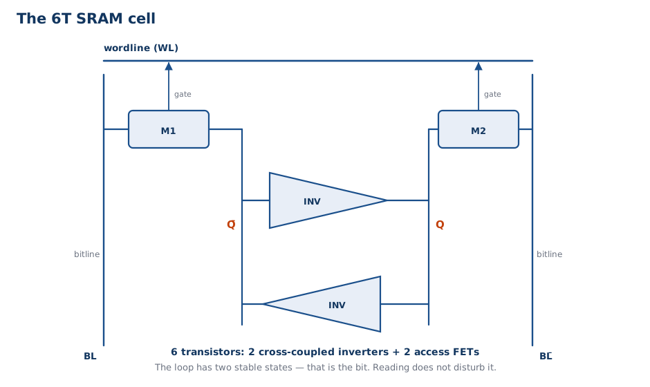
Six transistors, and the bit is held by feedback — no refresh, no capacitor, and reading it does not destroy it.

Draw this on the chalkboard rather than pointing at the ASCII. The key insight is “bistable”: two inverters in a ring have two fixed points, so the cell remembers.

Contrast with a latch: this is the same idea as the D-latch from the sequential logic deck, minus the clock, with the access transistors playing the role of the gate.

SRAM: Reading and Writing

Read — precharge both bitlines high and let them float, raise the wordline, and let the cell pull one bitline down. A sense amplifier resolves the small difference.

• The cell only pulls down; it never drives high. So the read is non-destructive.

Write — drive the bitlines hard to the desired values, raise the wordline, and overpower the cell’s feedback loop so it flips.

The access transistors must be sized so that a bitline at 0 can overpower a cell holding 1 — but a bitline at 1 must not overpower a cell holding 0.

Why the asymmetry? (Think about it before the next slide.)

MIT poses this as an open question on slide 6, and it is a genuinely good one. The answer: reads and writes share the same access transistors, and a read is just “let the cell fight the precharged bitline”. If the access transistor were symmetric and strong enough to write a 1 over a stored 0, then a read of a stored 0 would be flipped by the precharged-high bitline — reads would destroy data.

So the sizing is a compromise: strong enough to write, weak enough not to corrupt on read. Real designs use a write-assist (lowering the cell supply during write) to widen the margin.

Do not give the answer immediately — let them guess. It is the best discussion moment in Part I.

Why SRAM Cannot Be Large

Two limits, both physical:

1. Six transistors per bit. A 64 KB cache is half a million transistors before you count the tags, the decoders, or the sense amps.
2. Wires dominate. An N-entry multiported SRAM needs N wordlines and 2N bitlines crossing the array. The wire area grows as O(N²).

This is why “just make the L1 bigger” is not free, and why register files are tiny and multiported while caches are large and single-ported.

The O(N²) argument is MIT slide 7 and it is worth doing on the board: double the number of entries and the bitlines double in length and in count, so the wire area quadruples.

This is also the honest answer to “why is my L1 only 32 KB when I have 512 MB of RAM” — it is not cost, it is that the access time of a big array is set by the wire delay to the far corner.

DRAM: the 1T Cell

One transistor and one capacitor. The charge on the capacitor is the bit.

   wordline
      |
   BL ──[access]──┤├── ground
              (capacitor)

Consequences, all of them annoying:

• The capacitor leaks — every cell must be refreshed every few milliseconds.
• Reading shares charge between the capacitor and the bitline — so the read is destructive, and the value must be written back.
• The voltage swing is tiny, so every bitline needs a sense amplifier.

~20× denser than SRAM, and 2–10× slower. That is the trade, and it is a good one for main memory.

The capacitor is why DRAM is cheap: one transistor instead of six. The capacitor is also why DRAM is slow and complicated: leak, refresh, destructive read, sense amps.

The trench capacitor detail from MIT’s slide 9 is worth one sentence — to get enough capacitance in a small area you dig a deep trench or stack layers, which is a three-dimensional structure in a nominally planar process.

Flash and Disk

Flash — a floating gate traps electrons. Trapped charge means the transistor never inverts, so the cell reads as permanently off. No power needed to hold the bit.

• Very dense, non-volatile, no refresh
• Slow to write (10–100 µs), and writing damages the oxide: ~10³–10⁵ cycles

Disk — a magnetic domain, read by a head on a moving arm.

• ~10 ms to move the head: five orders of magnitude worse than DRAM
• But ~100× cheaper per bit, and it does not wear out

Flash and disk are why the hierarchy continues below DRAM — and why “swap” exists.

The endurance number matters practically: it is why SD cards die, and why the Debian image on their board runs from eMMC or an SD card rather than raw NAND.

Do not spend long here. The point is only that the hierarchy keeps going in both directions: registers above, flash and disk below.

Size Is a Fundamental Limit

“Size is a fundamental limit, even setting cost aside.”

Why: a bigger array means longer bitlines, which means more capacitance, which means a smaller voltage swing, which takes longer to sense.

Latency grows with capacity by physics, not by bad engineering. You cannot buy your way out of it with a bigger budget or a better process node.

So a large, fast memory is impossible. If we want the behaviour of one, we have to fake it — and that is what the rest of this lecture is about.

This is MIT slide 14 and it is the pivot of Part I. Everything before it was “why each technology is the way it is”; this is “and therefore the hierarchy is not optional”.

Say it plainly: there is no future process node at which a 512 MB SRAM with 1-cycle access appears. The wire delay alone forbids it.

…Unless You Stack It

The 2026 answer to “size is a fundamental limit” was not to scale the array. It was to put a second die on top of it.

AMD’s 3D V-Cache: a separate silicon die containing 64 MB of SRAM, bonded directly underneath the compute die and wired into the L3.

• Ryzen 7 9850X3D: 32 MB of on-die L3 + 64 MB stacked = 96 MB
• Same physics, different trick — the hierarchy got deeper by packaging

MIT’s 2017 deck says size is a fundamental limit. The industry’s response was to stop fighting it and start stacking.

This is the bridge into Part V and it is the most modern thing in the deck. The teaching point: the constraint from the previous slide is real, and engineers routed around it rather than through it.

Also worth noting the numbers for scale, which we will use again: 96 MB of L3 on that part, versus 512 MB of main memory on our board. Their cache is about a fifth the size of our entire DRAM.

Do not claim 3D V-Cache is transparent to software — it is, largely, but the OS needs to know which cores are near which cache. One sentence, move on.

Part II — Locality

The Locality Principle

Access to address X at time t implies access to X + ΔX at time t + Δt becomes more probable as ΔX and Δt approach zero.

Two special cases, and both matter:

• Temporal locality — ΔX = 0. You will touch the same address again soon.
• Spatial locality — Δt = 0. You will touch a nearby address soon.

This is an empirical claim about real programs, not a theorem. Compilers and programmers create it — and sometimes destroy it.

Read the statement carefully: it is a probability statement with two limits. MIT’s slide 17 states it exactly this way and the precision is the point.

Examples to give: temporal — a loop counter, a hot variable, an instruction in a loop body. Spatial — walking an array, fetching sequential instructions.

The “programmers can destroy it” line sets up conflict misses later: a pointer-chasing linked list has temporal locality but no spatial locality; a column-major walk of a row-major matrix has neither.

Reference Patterns and the Working Set

Plot address against time and real programs do not fill the space. They draw structured patterns, and each one is a different kind of locality:

• code (bottom) — ascending ramps: straight-line execution walking forward, then a branch back to the top of the loop. Each ramp is spatial locality; the ramps repeating at the same addresses is temporal locality.
• stack (middle) — drifts slowly upward in small clusters: frames pushed on a call, popped on return.
• data (top) — a handful of blobs that move around: a few live structures, not the whole array.

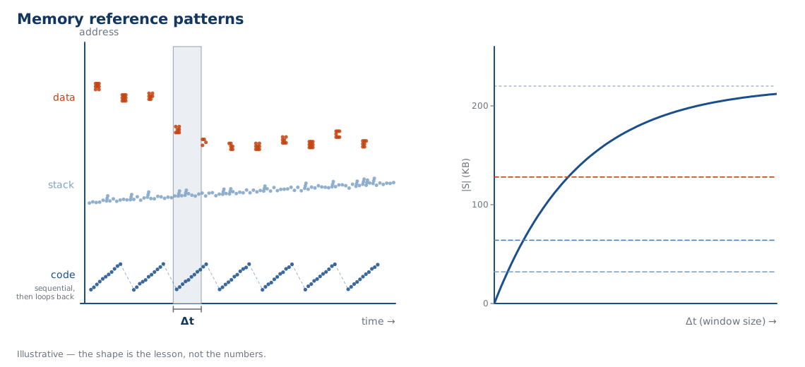
Pick a window Δt and count the distinct addresses touched. That set is the working set |S|. It grows with Δt, then saturates at the program’s real footprint.

That saturation is the whole opportunity: a cache bigger than the saturated working set sees mostly hits.

MIT slide 18. The graph is the important artefact — address on the vertical axis, time on the horizontal, and the accesses forming clumps rather than a uniform fog.

Walk the three motifs explicitly, because they are three different phenomena:

• The code ramps are the best one. Execution walks forward through instructions (the ramp), hits a branch, and jumps back (the drop). Then it runs the same ramp again, at the same addresses. That single shape contains both halves of the locality principle.
• The stack clusters are call/return: push frames on the way down, pop on the way up. It drifts because the stack grows and shrinks around a moving base.
• The data blobs are the point students miss: a program touching 512 MB of DRAM does not touch it evenly. At any moment it is working on a few structures, and the blobs show which.

The saturation is the punchline. It says the working set is bounded even though the program runs for an unbounded time. That is why a 64 KB cache can serve a program that touches gigabytes.

Ask the class: what does the curve look like for a program that streams a 3 MB video frame once? Answer: |S| never saturates — no reuse, so no locality, and the cache cannot help. That is exactly why the engines use DMA and carveouts instead (see the power deck).

Everything Is a Cache for Something Else

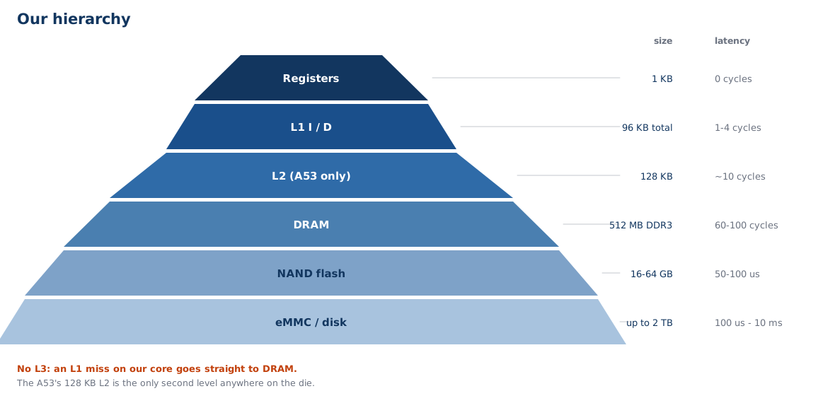
Each level is a cache for the level below it — and each has a different owner: the compiler allocates registers, hardware manages the caches, the OS runs the flash page cache. Same problem, three different owners.

This is MIT slide 20 with our column filled in, and the filled-in column is the slide’s value: no L3, and an L2 that exists on only one of the four cores.

The “managed by” column is the one students have not thought about. Registers are allocated by the compiler — that is a cache replacement policy implemented in software, and it is why register allocation is a hard compiler problem. Flash-to-DRAM is managed by the OS page cache. Same problem, three different owners.

Expose or Hide?

Two ways to give a programmer a hierarchy:

Expose it. “Here are two memories. Put the hot data in the fast one yourself.” Scratchpad memory, DSPs, some GPUs, and — partly — our ION carveouts.

Hide it. One flat address space. Hardware (and the OS) decide where data lives. That is a cache.

Every real system does both. Ours does both: the caches hide, and the carveouts expose.

MIT slides 15–16 frame this as the interface question, and it is a good one because it is a design choice with no universally right answer.

Exposed memory is predictable — a scratchpad has no conflict misses, so a real-time audio pipeline can bound its worst case. Hidden memory is easier to program and usually faster on average.

Tie to our board: ION carves DRAM out and hands it to the video pipeline as physically contiguous buffers. That is an exposed hierarchy: the driver decides what goes there. The caches are the hidden half. Students saw this in the power deck; this is the same idea from the other direction.

Part III — AMAT: The One Equation

Hit, Miss, and Two Ratios

A cache is asked for an address. There are exactly two outcomes:

Outcome	What happens	Cost
Hit	the block is present; return it	hit time (a few cycles)
Miss	not present; fetch the block, evict something, return it	hit time + miss penalty

• Hit ratio (HR) = hits / total accesses
• Miss ratio (MR) = 1 − HR

The processor now has variable memory access time, and something has to cope with that — either stall the pipeline, or keep going out of order.

This is MIT slide 21. The point about variable latency is the one students underrate: a cache turns a fixed-cost memory into a variable-cost memory, and the whole microarchitecture has to absorb the variance. That is why an in-order core with a cache miss is so much slower than an out-of-order one.

Our C906 is in-order. A miss there is a hard stall — no other work to do. Worth saying, and worth connecting to the pipelining material.

AMAT

The average memory access time:

\[\text{AMAT} = \text{HitTime} + \text{MissRatio} \times \text{MissPenalty}\]

Read it as: every access pays the hit time, and a fraction of them pay the penalty on top.

Two reasons this is the right metric:

• It is per access, so it multiplies cleanly by the instruction count.
• It composes — the miss penalty of one level is the AMAT of the next.

Do not let them memorise this without understanding the shape. The key structure: hit time is paid unconditionally; the penalty is paid conditionally.

A useful sanity check to do on the board: if HR = 1, AMAT = HitTime. If HR = 0, AMAT = HitTime + MissPenalty, which should equal the raw memory latency — and it does, if HitTime is small relative to the penalty.

AMAT is what MIT slide 22 introduces and returns to on slides 28, 34, and 40. It is the spine of the lecture; point that out so they notice the recurrence.

AMAT Composes

The miss penalty of level 1 is the AMAT of level 2:

\[\text{AMAT} = \text{HT}_1 + \text{MR}_1 \times \bigl(\text{HT}_2 + \text{MR}_2 \times \text{Penalty}_{\text{mem}}\bigr)\]

Now apply it to our two big cores, with the same L1 hit ratio of 0.95:

Core	Hierarchy	AMAT
C906	L1 → DDR3	2 + 0.05 × 80 = 6.0 cycles
A53	L1 → L2 → DDR3	2 + 0.05 × (10 + 0.20 × 80) = 3.3 cycles

Same L1. Same hit ratio. The L2 nearly halves the AMAT — because it catches most of the 5% that miss L1.

This is the most important quantitative slide in the deck, because it explains why the A53 feels so much faster than the C906 at the same clock and with the same L1 sizes.

Walk the arithmetic slowly. Inside the bracket: a miss in L1 costs the L2 hit time (10) plus, 20% of the time, the full memory penalty (80). That is 10 + 16 = 26. Multiply by the 5% L1 miss rate: 1.3 cycles on top of 2.

For the C906 there is no bracket — the 5% miss pays the whole 80 cycles.

The numbers 10 and 80 are illustrative, not measured. The structure is the lesson: a second level exists to shorten the bracket.

What Hit Ratio Do You Need?

Suppose a hit costs 2 cycles and a miss costs 100.

Target	Equation	Required HR
Beat no cache at all (AMAT < 100)	100 = 2 + (1−HR)·100	2%
AMAT = 10 cycles	10 = 2 + (1−HR)·100	92%
AMAT = 5 cycles	5 = 2 + (1−HR)·100	97%

Even a terrible cache beats no cache. But a good one has to be very good indeed — the last few percent of hit ratio is where all the engineering lives.

MIT slide 23 uses 4 cycles for a hit and 100 for a miss, giving 4% and 99%. Our hit time is lower, which lowers the bar: 2% instead of 4%. Show that the break-even point is just HitTime / MissPenalty — so a faster hit time makes the cache more forgiving.

The pedagogical shape is the non-linearity: going from 92% to 97% only buys 5 cycles, but going from 0% to 2% buys 98. Diminishing returns, which sets up the associativity curve in Part IV.

The Honest Caveat

That “80 cycles” is an estimate, not a measurement. It is DDR3 CAS latency plus tRCD plus controller scheduling, and the controller is allowed to reorder.

• Bandwidth floor: one 64-byte line at peak 1866 Mbps × 16 bit = 3.73 GB/s is 64 B ÷ 3.73 GB/s ≈ 17 ns ≈ 17 cycles at 1 GHz.
• Latency is several times that, because a single random read cannot use peak bandwidth.

We do not need the exact number to reason about caches. We need the shape: hit time is single digits, miss penalty is double digits.

Be explicit that this is derived, not measured. The bandwidth figure is solid arithmetic (1866 Mbps × 16 bits); the latency figure is an engineering estimate.

The distinction between latency and bandwidth is the thing to teach here, because students conflate them constantly. Peak bandwidth is what you get with a long stream of sequential requests; latency is what you pay for one lonely cache line. A cache miss is the second case, so the bandwidth number is a lower bound on the cost, not an estimate of it.

If anyone asks how you would actually measure it: that is the lab, and we are not doing the lab today.

Part IV — How a Cache Works

The Basic Algorithm

on each access to address A:
    if the cache holds the block containing A:
        HIT   → return the data, a few cycles
    else:
        MISS  → choose a line to evict
              → fetch the block containing A from memory
              → place it in the cache
              → return the data

The pseudocode hides the two questions that define a cache:

1. How do we search? → direct-mapped, set-associative, fully-associative
2. Which line do we evict? → the replacement policy

MIT slide 24 ends with exactly this question: “How do we search the cache?” That is the pivot into the next four slides.

Everything in Part IV is an answer to question 1 or question 2. Say that explicitly, so the section has a spine and is not a list of vocabulary.

There is a third question — when do we write to memory — which is the write policy, later.

Direct-Mapped: the Simplest Search

One place for each block. Block number modulo the number of lines.

Each line stores a valid bit, a tag, and the data:

index	valid	tag	data
0	1	0x20000	64 bytes
1	0	—	—
2	1	0x1F4A3	64 bytes
…
255	1	0x20001	64 bytes

Search: index the array, compare one tag. That is a single comparator, not a search.

The genius of direct-mapped is that “search” degenerates to “compute an address and check one tag”. No comparators, no mux, no CAM. That is why it is fast and cheap.

Note the valid bit: on reset every tag is garbage, so the valid bit is what says “trust me”. Emphasise it — students forget it and then cannot explain a cold-start miss.

A Worked Lookup on Our D-Cache

Our L1 D-cache: 64 KB, 4-way, 64 B lines ⇒ 256 sets. A 32-bit address splits as tag 18 | index 8 | offset 6.

Address	offset	index	tag	Result
0x8000_1040	0x00	0x41 (65)	0x20000	load it into set 65
0x8000_1040 again	0x00	0x41	0x20000	HIT
0x8000_5040	0x00	0x41	0x20001	different tag — MISS

Both addresses land in set 65. In a direct-mapped cache they would evict each other forever. In ours, both can live there — we have four ways.

Do this arithmetic live on the board; it is the single most useful mechanical skill in the lecture. Write the address in binary, slice 6 bits off the bottom, then 8, and everything left is the tag.

Check the second row explicitly: 0x8000_5040 − 0x8000_1040 = 0x4000 = 16384 = 256 × 64. So the two addresses are exactly 256 lines apart, which is why the index is identical.

The punchline is the fragment: this is a conflict, and associativity is the cure.

Part of the Address Is Encoded in the Location

The index bits are not stored anywhere. They are implied by which line you looked in — the hardware computed them from the address.

So the tag array only needs the top bits:

Cache	Sets × ways	Metadata per line	Tag array total
Direct-mapped 64 KB	1024 × 1	18 tag + 1 valid + 1 dirty	640 B
Our 4-way 64 KB	256 × 4	18 tag + 1 valid + 1 dirty	2.5 KB

The address is partly stored in the location. That is what makes a cheap, one-comparator search possible — and it is also the source of conflict misses.

MIT slide 26 puts this in a red banner and it deserves the emphasis: “Part of the address (index bits) is encoded in the location!”

The arithmetic: 256 sets × 4 ways × 20 bits = 20,480 bits = 2.5 KB, on top of 64 KB of data. About 4% overhead. A direct-mapped cache of the same size needs only 640 B — a quarter of the metadata, for a quarter of the flexibility.

This is also the intuition for why the tag can be small: 18 bits instead of a 32-bit address.

Block Size: the Third Field

The address now has three fields, not two:

 31                    14 13        6 5      0
+------------------------+-----------+--------+
|         tag (18)       | index (8) | off (6)|
+------------------------+-----------+--------+

The block offset selects a byte inside the line. It costs nothing to store — it is pure address arithmetic — and it buys you spatial locality for free.

So why not make blocks enormous? Because a bigger block means:

• fewer blocks for the same capacity → more conflicts
• a longer fill: you must fetch the whole line before you can use any of it
• wasted bandwidth if you never touch the rest of the line

The three-field split is the single diagram to leave on the board for the rest of the lecture. Everything else is a variation on it.

The “costs nothing to store” point is subtle and worth making: the offset bits are not in the tag array, so a 64-byte block is 64× the data for the same tag storage. That is why blocks exist at all.

The three costs in the fragment are the setup for the next slide’s U-curve.

Block Size Tradeoffs

AMAT is U-shaped in block size, because two effects fight: bigger blocks cut the miss rate (more spatial reuse per fetch) but raise the miss penalty (a longer fill before you can use any of it).

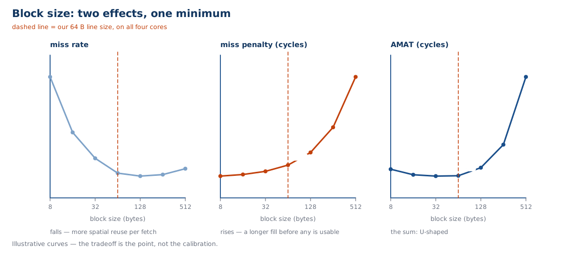
MIT’s deck puts the optimum at about 64 bytes (slide 28). Our C906’s line size is exactly 64 bytes, on both caches.

That is not a coincidence. It is the same optimum, found independently.

MIT slide 28 shows three curves — miss rate falling, miss penalty rising, and AMAT U-shaped between them — with the minimum around 64 bytes. Draw the two components and let the sum appear.

The reason the optimum is so stable across machines is that it is set by DRAM burst length and by the granularity of spatial locality in real code, not by the cache.

Land the point: our hardware agrees with the textbook, which should increase their confidence in the textbook. Later we will find places where it does not.

Conflict Misses

Misses come in three kinds:

• Compulsory (cold) — first touch. Unavoidable.
• Capacity — the working set is bigger than the cache. Unavoidable at that size.
• Conflict — the working set fits, but maps to too few sets. Avoidable.

A concrete case on our D-cache. A row of this matrix is exactly 16 KB:

int A[1024][4096];        /* 4096 ints = 16 KB per row */
for (int i = 0; i < 1024; i++)
    sum += A[i][0];       /* walk one column */

Every A[i][0] is 16 KB after the last — 256 lines apart — so they all land in the same set. Four fit in four ways. The fifth thrashes, forever.

This is MIT slide 29’s lesson (their version: two data arrays 1024 words apart all hit; 2048 words apart all miss) translated into our geometry, where the magic stride is 16 KB = 256 sets × 64 B.

The fix, for the record, is to pad the row length or transpose the loop. Say it, but do not dwell — the point is that the programmer can create or destroy locality, which recalls the Part II warning.

Ask: how many ways would you need to survive this? Answer: 1025 — i.e. fully associative, i.e. the wrong fix. The right fix is to change the access pattern.

Fully Associative

No index at all. A block may live in any line.

To search, compare the tag against every line in parallel — that is a CAM, and it costs one comparator and one tag read per line.

	Direct-mapped	Fully associative
Search cost	1 comparator	N comparators
Conflict misses	many	none
Data select	none	N:1 mux

Used where N is small and misses are expensive: our μTLBs are 10-entry fully associative, and the branch target buffer is 16-entry fully associative.

The CAM cost is the whole story: you cannot build a 256-entry fully associative cache without 256 parallel comparators on the critical path, which is why real L1 caches are never fully associative.

But our C906 does use it where it fits — the I-μTLB and D-μTLB are 10 entries each, fully associative, and the BTB is 16 entries. Those are small enough that N comparators is affordable, and misses there are expensive enough to be worth it.

Nice moment: the same design decision, made three times at three different scales on the same core.

N-Way Set Associative

The compromise. Draw the cache as a grid:

          way 0      way 1      way 2      way 3
set 0   [ v|tag|d ] [ v|tag|d ] [ v|tag|d ] [ v|tag|d ]
set 1   [ v|tag|d ] [ v|tag|d ] [ v|tag|d ] [ v|tag|d ]
set 2   [ v|tag|d ] [ v|tag|d ] [ v|tag|d ] [ v|tag|d ]
  ...      ...        ...         ...         ...
set 255 [ v|tag|d ] [ v|tag|d ] [ v|tag|d ] [ v|tag|d ]

A block maps to one row (chosen by the index) and may occupy any column.

Direct-mapped is 1-way. Fully associative is 1 set.

It is exactly N direct-mapped caches in parallel, sharing an index.

This is MIT slides 31–32. The grid is the right mental picture and it is worth drawing properly: rows are sets, columns are ways, and a cache lookup touches an entire row.

The two degenerate cases are the point: the space of designs is one parameter, N, with direct-mapped at one end and fully associative at the other. Students who see it that way stop memorising three separate structures.

N-Way Structure

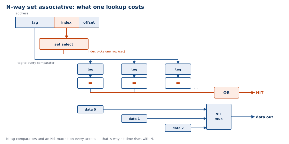
Cost: N comparators and an N:1 mux on the critical path. Hit time grows with N.

That is the tension: more ways means fewer conflict misses, but every access pays for the extra comparators.

The structure diagram explains the whole tradeoff in one picture: the comparators are in parallel, so the delay is not N× a comparator, but it is an N-input OR tree plus an N:1 mux, and both get slower as N grows.

Say clearly: this is why associativity is not free, and why the AMAT curve in the next slide has a minimum rather than falling forever.

Associativity Tradeoffs

AMAT versus associativity is also U-shaped: conflict misses fall, hit time rises.

“Little additional benefit beyond 4 to 8 ways.” — H&P, cited on MIT slide 34

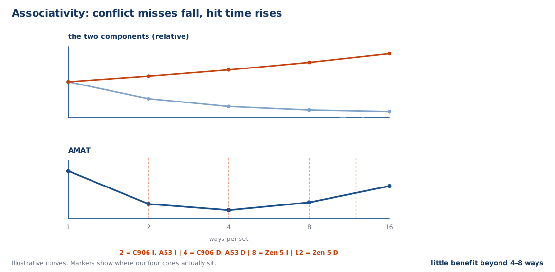
All four of our cores sit on that curve. Zen 5 raised its L1 D-cache from 8-way to 12-way specifically to accommodate the larger 48 KB size — the tradeoff, visible in a shipping product.

MIT slide 34 is H&P Figure 5.9, and the quotation is the takeaway: beyond 4 to 8 ways you are paying hit time for a shrinking benefit.

The Zen 5 detail is a lovely confirmation: AMD did not go to 12 ways for fun, they went because they wanted 48 KB and 8-way would have made the conflict rate worse. That is exactly the reasoning the lecture just taught, in a product launched in 2026.

The A53 row is the interesting one: 2-way instruction, 4-way data — identical to the C906. Two vendors, two ISAs, one die, the same asymmetry. The next slide argues about why.

Replacement Policy

Only matters when ways > 1 — you must choose a victim.

Policy	Rule	Cost
Belady’s MIN	evict the block used furthest in the future	optimal; needs the future — unimplementable
LRU	evict the least recently used	good; needs ~log₂(N!) bits per set
FIFO	evict the longest-resident	cheap; log₂(N) bits — but not a stack algorithm
Random	evict at random	no state; no adversarial pattern

Belady’s MIN is still useful: it is the lower bound you measure other policies against.

And no core on our board implements true LRU — the C906 uses FIFO, the A53 uses pseudo-random, x86 uses an approximation. The textbook policy is the reference, not the implementation.

MIT slide 36. The classification worth remembering: Belady is a bound, LRU is the quality reference, FIFO and random are the cheap approximations.

Exact LRU for a 4-way set needs enough state to encode one of 4! = 24 orderings, i.e. 5 bits; FIFO needs 2. That is the cost side. Real hardware mostly uses pseudo-LRU approximations because true LRU’s bookkeeping is on the critical path.

Foreshadow: our C906 uses FIFO on both caches, and that has a consequence we will look at in Part V. The A53 next to it uses pseudo-random, which has no recency information at all but also no adversarial pattern. Neither is LRU — that is a textbook idealisation, not something you can buy.

Why FIFO Is Different

FIFO is not a stack algorithm — it does not obey the inclusion property. The consequence is Belady’s anomaly: giving it more capacity can make it worse.

Classic reference string, three frames versus four:

Frames	Faults
3	9
4	10

More cache, more misses. LRU cannot do this — it is a stack algorithm, so a bigger cache always contains the smaller one’s contents.

In practice FIFO is usually fine. But “usually fine” is a different claim from “cannot be worse”, and our D-cache makes the weaker one.

The reference string is 1 2 3 4 1 2 5 1 2 3 4 5. Walk it on the board if there is time — it takes two minutes and students remember it for years, because it violates the intuition that more memory is always at least as good.

Be fair to our hardware: Belady’s anomaly is a capacity effect, and in a fixed 4-way cache it is a curiosity rather than a practical problem. The honest statement is that FIFO gives up a guarantee LRU has, and gains cheap bookkeeping in exchange.

This is the slide where “our silicon differs from the textbook” first bites, so it is the natural bridge into Part V.

Write Policy

Reads are easy. Writes force a choice — and a second one on a write miss:

Policy	On a write	Cost
Write-through	write cache and memory	simple, no dirty bit — but every store costs bandwidth
Write-behind	write a buffer, drain later	core does not stall; still full bandwidth
Write-back	write only the cache; memory on eviction	fastest, lowest bandwidth — needs a dirty bit

And on a write miss: write-allocate (fetch the block first) or write-no-allocate (write straight through)?

Our C906 D-cache: write-back, with write-allocate / write-no-allocate configurable — and an adaptive mode we will meet in Part V.

MIT slide 37 presents the three policies with write-back marked “commonly implemented”, which is still true.

The second question — allocate or not on a write miss — is the one that matters more in practice and gets less attention. If you are going to overwrite the entire line, fetching it first is pure waste: you pay a memory read for data you are about to destroy. That is why streaming stores exist, and why our chip has an adaptive mechanism.

Draw the connection: memset of a large buffer is the pathological case for write-allocate.

Dirty Bits

One extra bit per line. It answers: does memory match this line?

• WRITE to a line → set dirty = 1
• Evict a line → write it back only if dirty == 1
• Fill a line from memory → dirty = 0

The consequence is uncomfortable: main memory can be stale. DRAM is not the truth; the cache is. Everything that bypasses the cache — DMA, another core, a debugger — now has a coherency problem.

This is MIT slides 38–39, and it is where the lecture connects to the power deck’s DMA material.

The uncomfortable consequence is the important one. Once you have a write-back cache, “the value in memory” is a lie, and every agent that reads memory without going through the cache has to be told. That is what dma_sync_* does in Linux, and it is why the little C906 being non-coherent with the big core matters.

Also: this is why cache maintenance instructions exist at all — DCACHE.CPA, DCACHE.CIPA, ICACHE.IVA and friends. They are the manual override for “make memory true again”. We are not doing the lab, but that is what they are for.

Part V — Four Cores, Four Answers

Four Cores, Four Answers

Everything so far was the model. Here is what four real cores did with it.

	C906 @ 1 GHz	C906 @ 700 MHz	Cortex-A53	Ryzen 7 9850X3D
L1 I	32 KB, 2-way	16 KB, 2-way	32 KB, 2-way	32 KB, 8-way
L1 D	64 KB, 4-way	16 KB, 4-way	32 KB, 4-way	48 KB, 12-way
L2	—	—	128 KB, 16-way	1 MB, 16-way
L3	—	—	—	96 MB
Line	64 B	64 B	64 B	64 B
Replacement	FIFO	FIFO	pseudo-random	n/d
Prefetch	yes, both	yes, both	n/d	yes

Associativity runs 2 → 4 → 8 → 12. L3 runs none → none → none → 96 MB.

But look at the first two columns of associativity: the C906 and the A53 are identical — 2-way instruction, 4-way data. And the line size is 64 bytes on all four. Two of those columns are industry consensus.

This is the payoff slide for the whole lecture. Every column is a design decision the students can now name and justify.

The 64-byte line across all four is the strongest evidence for the block-size slide: it is set by DRAM burst granularity and by the spatial locality of real code, and it has been stable for two decades.

Two honesty notes. n/d means not documented in the sources we had — AMD’s replacement policy is not published in a citable form. A dash (—) means the level does not exist. Keep those two symbols distinct; conflating them is how spec tables lie.

The A53 row comes from Arm’s Cortex-A53 TRM. Note that its L1 geometry matches the C906’s exactly: 2-way instruction, 4-way data. That is the finding this slide was missing — see “Two Vendors, One Answer”.

Two C906s, Not One

The SG2000 has two C906 cores, and they are not the same core:

	Big C906	Little C906
Clock	1.0 GHz	700 MHz
L1 I	32 KB	16 KB
L1 D	64 KB	16 KB
Runs	Linux	FreeRTOS / bare metal
MMU	yes	M-mode, physical

Half the clock — but half the I-cache and a quarter of the D-cache. A memory-bound workload on the little core loses far more than 30%: it loses on capacity and on latency at the same time.

This is a distinction students routinely miss — they see “2 × C906” in the SG2000 summary and assume two identical cores. The 700 MHz part has a much smaller cache, and that is a bigger deal than the clock.

Note the trap: 700/1000 = 0.7, so a compute-bound workload loses 30%. But a memory-bound workload loses more, because the smaller cache raises the miss ratio while the slower clock raises the cycle time. Both penalties compound.

Also: the little core runs M-mode with physical addressing, so it has no MMU and no TLB pressure — which means its cache behaviour is, if anything, simpler to reason about than the big core’s.

C906 L1 I-Cache: 2-Way

Straight from the manual (§7.1):

Property	Value
Size	8 / 16 / 32 / 64 KB, hardware-configurable
Associativity	2-way set associative
Line	64 B
Indexing	VIPT — virtual index, physical tag
Read width	32 bits
Refill width	128 bits
Replacement	FIFO
Maintenance	whole-cache and single-line invalidate
Prefetch	yes — MHINT.IPLD, same page only

2-way is the bottom of the useful range — the minimum that removes the worst conflict misses without paying for comparators on the fetch path.

Walk the table. Two entries deserve comment.

The 32-bit read width with a 128-bit refill means the I-cache is filled four words at a time but read one word at a time — a deliberate asymmetry, because refills are bandwidth-bound and fetches are latency-bound.

The prefetch restriction to the same page is a safety feature: prefetching across a page boundary could touch an address with no valid mapping. That is a correctness constraint, not a performance one, and it is a nice example of a cache interacting with virtual memory.

2-way is unusual for an I-cache. Note it and move on — the discussion comes in two slides.

C906 L1 D-Cache: 4-Way

§7.2 — and note how much more there is to say than for the I-cache:

Property	Value
Size	8 / 16 / 32 / 64 KB, hardware-configurable
Associativity	4-way set associative
Line	64 B
Indexing	VIPT
Read / write width	64 bits / 128 bits
Write policy	write-back, write-allocate or write-no-allocate (configurable)
Replacement	FIFO
Prefetch	sequential and strided (stride ≤ 16 lines, forward and backward)
Extra	adaptive write-allocate; LR/SC local monitor

The D-cache is where the interesting engineering is. Every row past “line size” is an optimization the I-cache does not need.

The contrast with the previous slide is the point: the data side has five extra mechanisms, because data access patterns are varied and instruction access patterns are not.

The 128-bit write width matters for a different reason than the read width: it lets the core commit two registers per cycle into the cache, which is what an in-order core needs to keep a store pipeline busy.

Bidirectional strided prefetch is genuinely unusual — most prefetchers only go forward. Backward prefetch helps with loops that walk down an array.

Mention LR/SC briefly: it is implemented as a monitor inside the L1 D-cache, and it fails if the D-cache is disabled. That is a lovely example of an unrelated feature (atomic operations) silently depending on a cache being switched on.

Two Vendors, One Answer

The C906 splits its Harvard cache: I-cache 2-way, D-cache 4-way.

The Cortex-A53 — different vendor, different ISA, same die — splits it exactly the same way:

	L1 I	L1 D
C906 @ 1 GHz	32 KB, 2-way	64 KB, 4-way
Cortex-A53	32 KB, 2-way	32 KB, 4-way

Neither manual explains the choice. But two independent design teams landing on 2/4 is not a coincidence — it is a consensus, and consensus usually has a reason.

Two hypotheses, and they are not mutually exclusive:

• The I-cache sits on the fetch critical path — every comparator added there delays every instruction fetch, so it is kept minimal.
• Instruction streams are regular and sequential with few conflicts, so the extra ways buy less on the I side than on the D side.

This is the intellectual centre of Part V, and it got stronger once we filled in the A53. It is no longer “one vendor was inconsistent” — it is two vendors, two ISAs, one die, arriving at the same asymmetry independently.

That turns a curiosity into evidence. If one team chose 2/4 you could dismiss it as habit; when two do, the asymmetry is probably real engineering.

Do not give them an answer, because we do not have one — neither manual states a rationale, and inventing one would teach them to make things up.

A good prompt if the room is quiet: what would you expect on a core with a trace cache or a very wide fetch? (The I-side gets more pressure, so the asymmetry should grow.)

The A53 Has an L2. We Don’t.

	C906 @ 1 GHz	Cortex-A53 @ 1 GHz
L1 I	32 KB, 2-way	32 KB, 2-way
L1 D	64 KB, 4-way	32 KB, 4-way
L2	none	128 KB, 16-way
On an L1 miss	straight to DDR3	L2 first

Back to the AMAT composition, same 0.95 L1 hit ratio:

	AMAT
C906: 2 + 0.05 × 80	6.0 cycles
A53: 2 + 0.05 × (10 + 0.20 × 80)	3.3 cycles

Identical associativity. Identical line size. The C906 even has twice the L1 D-cache — and it still loses, because there is nothing behind it to absorb a miss.

This is the single most practically useful comparison in the deck, and it is not the one students expect. The two cores have the same associativity and the same line size, and the C906 has more L1 data cache — and it is still the slower core for memory-bound work. The only variable left is the L2.

That is what makes it a clean experiment rather than a pile of differences.

The lesson: L1 capacity and L2 presence are not interchangeable, and the second level is worth more than extra first-level ways or kilobytes, because it attacks the penalty term rather than the miss rate.

Caveat clearly: 10 and 80 are illustrative. The structure is the claim, not the digits.

Our Bit Arithmetic

Apply the three-field split to all four of our caches. Line size is 64 B everywhere, so the offset is always 6 bits:

Core	Cache	Size	Ways	Sets	index	offset	tag
C906 1 GHz	I	32 KB	2	256	8	6	18
C906 1 GHz	D	64 KB	4	256	8	6	18
C906 700 MHz	I	16 KB	2	128	7	6	19
C906 700 MHz	D	16 KB	4	64	6	6	20

Both 1 GHz caches land on 256 sets and 8 index bits — different sizes, same geometry. The 64 KB D-cache gets its extra capacity from the fourth way, not from more sets.

The arithmetic: sets = size ÷ (ways × line). 32768 ÷ (2×64) = 256. 65536 ÷ (4×64) = 256. 16384 ÷ (2×64) = 128. 16384 ÷ (4×64) = 64.

The coincidence on the third row is genuinely useful pedagogically: the 1 GHz I and D caches have the same index width, so the same address maps to the same set number in both — which is irrelevant because they are separate caches, but it makes the point that capacity can be bought with ways as well as with sets.

Two honesty notes. First, the C906 is RV64, so with a full 64-bit address the tag is 50 bits, not 18 — we use 32-bit addresses here to match the rest of the deck. Second, these are derived numbers, not quoted from the manual; the manual gives sizes, ways, and line size, and the rest is arithmetic.

VIPT: Why the Index Can Be Virtual

VIPT = virtual index, physical tag. Why bother?

virtual address ──┬──► [ index ] ──────────────► select set  ──┐
                  │                                            ├──► compare
                  └──► [ TLB ] ──► physical ──► [ tag ] ───────┘
                                    (in parallel)

The index needs no translation, so the TLB lookup and the set selection run at the same time. With a physical index you would have to translate first, then index — two serial latencies on every access.

The constraint: the index bits must lie entirely inside the page offset. Otherwise two virtual addresses for the same physical page could pick different sets — synonyms.

\[\text{sets} \times \text{line size} \le \text{page size}\]

VIPT is the concrete instance of MIT’s “part of the address is encoded in the location” — and it is why that slogan has teeth. The index is computed from the virtual address before anyone knows what physical page it is in.

Draw the two paths: the index path is short and goes straight to the SRAM; the tag path goes through the TLB. They meet at the comparator. That is the whole trick, and it is worth a proper diagram on the board.

The constraint in the box is the one that bites on the next slide.

The Open Question

Our 1 GHz caches: 256 sets × 64 B = 16 KB. Our small page size: 4 KB.

\[16\ \text{KB} > 4\ \text{KB}\]

So two of the eight index bits come from the virtual page number, not from the page offset. Which means the hardware is either:

1. using “VIPT” loosely, and cacheable mappings must use ≥ 16 KB pages;
2. doing something undocumented to handle synonyms; or
3. accepting aliasing, and relying on the OS never to create it.

The manual does not say. We do not know. This is a real, checkable open question about the chip in your hand — and a good one.

Be scrupulous here: this is our derivation from two documented facts (the cache geometry in §7.2 and the 4 KB page size in the MMU chapter), not a claim the manual makes. The manual says VIPT; the arithmetic says the constraint is violated at 4 KB.

The most likely reading is (1) — cacheable regions use larger pages, and the MMU supports 2 MB and 1 GB pages, which would make the constraint comfortably satisfied. But “most likely” is not “documented”, and saying so out loud is better teaching than smoothing it over.

This is also a good exam question or a project: write a test that maps two virtual addresses to the same physical page and measures whether the cache aliases.

Write-Back, Prefetch, and Adaptive Allocation

Three mechanisms on our D-cache that MIT’s taxonomy does not contain:

• Write-back with a dirty bit — exactly as taught, no surprise.
• Strided prefetch — the LSU detects a miss pattern and prefetches up to 16 lines ahead, forward or backward. It manufactures spatial locality that is not there.
• Adaptive write-allocate — after N consecutive line writes (HINT.AMRL1), the page’s write-allocate property switches off automatically.

That last one is the memset problem, solved in hardware: if you are writing a whole buffer, fetching each line before overwriting it is pure waste. The cache notices and stops doing it.

This slide is the best answer to “why should I care about the textbook model if real chips differ” — because the differences are all refinements of the model, and you cannot see why they exist until you know what problem they solve.

Adaptive write-allocate is the clearest case. From the textbook you learn write-allocate versus write-no-allocate is a static configuration choice. Real hardware makes it dynamic, per page, based on observed behaviour, because neither static choice is right for all code.

The prefetcher is worth a caveat: prefetching manufactures locality, which means the locality principle is no longer purely an empirical fact about programs — hardware now exploits access patterns that a naive working-set analysis would call random.

Part VI — Synthesis

What We Actually Learned

1. The hierarchy is forced. A large fast memory cannot be built — latency grows with array size by physics. Stacking dies is the only recent escape.
2. Locality is the load-bearing assumption. If programs accessed memory uniformly, every technique here would be worthless.
3. AMAT is the whole game. HitTime + MissRatio × MissPenalty. Every mechanism in the lecture moves one of those three terms.
4. Associativity, block size, and replacement are three answers to two questions. How do we search, and whom do we evict.
5. Our four cores are all on the same curves — 2, 4, 8, 12 ways; 64-byte lines; none to 96 MB of L3.

The textbook model is not wrong. It is under-specified — and the places where real silicon fills in the gaps are exactly where the engineering lives.

Read these as the examinable summary. Each one is a sentence a student should be able to expand into a paragraph.

Claim 5 is the one that took the whole of Part V to establish, and it is the one worth the most: they should leave able to look at any processor’s spec sheet, read the cache line, and say something intelligent about it.

Discussion Prompts

• Both the C906 and the A53 are 2-way on instructions and 4-way on data. Argue for or against keeping the two sides symmetric — and say what evidence would settle it.
• The A53 has 32 KB + 32 KB + 128 KB; the C906 has 32 KB + 64 KB and no L2. Which would you rather compile for, and does the answer depend on the program?
• Adaptive write-allocate turns itself off under streaming stores. What could go wrong with a mechanism that changes policy based on observed history?
• The VIPT constraint appears to be violated at 4 KB pages. Design an experiment that would settle it.
• Given AMAT = HT + MR × MP, and a fixed transistor budget, where do you spend it — more ways, more sets, or an L2?

Every one of these is answerable from the material in this deck. None has a single right answer.

These are designed to be argued in class or written as homework. The last one is the best: it forces them to use the equation rather than recite it.

For the fourth, the experiment is: allocate two virtual pages, map them to the same physical page, write through one and read through the other, and see whether the second read sees the first write. If it does, no aliasing. That is a real test and it is within reach of someone who can write a kernel module.

Do not answer them. Let the room do it.

Refs

Primary sources for this deck

• XuanTie C906 User Manual (openc906), §7 memory subsystem, §5 MMU, §7.3 cache operations — the L1 geometry, FIFO policy, and prefetch mechanisms.
• SG2000 / SG2002 Technical Reference Manuals — the core configurations and the address map.
• MIT 6.004 Computation Structures, Spring 2017, lecture 14 — the structure of the stock story, and the AMAT framing.
• Hennessy & Patterson, Computer Architecture, cache chapter — associativity tradeoffs, replacement policies.
• AMD Zen 5 microarchitecture tables and the Ryzen 7 9850X3D product page — the x86 comparison.

Point them at refs.md for the condensed version with the full numbers and the per-claim sources.

Be explicit that the C906 numbers come from the vendor manual and the derived numbers (the bit arithmetic, the AMAT examples) are ours — so they know which ones to trust and which ones to check.